Envelope of projectile motion

Envelope of projectile motion

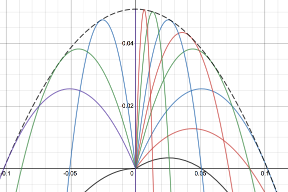
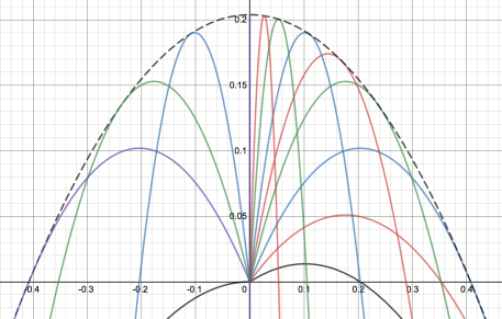
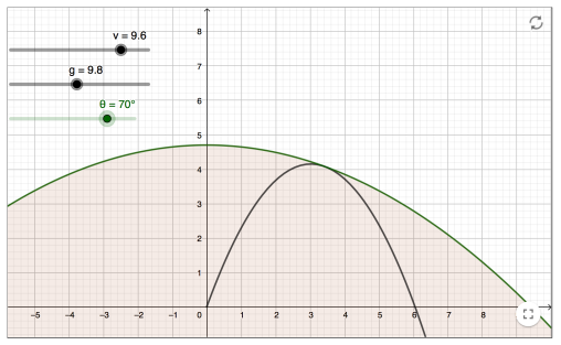
For any given launch angle and for a fixed initial velocity we will get projectile motion. In the graph above I have changed the launch angle to generate different quadratics.  The black dotted line is then called the envelope of all these lines, and is the boundary line formed when I plot quadratics for every possible angle between 0 and pi.

Finding the equation of an envelope for projectile motion 

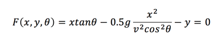
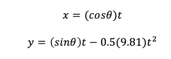
Let’s start with the equations for projectile motion, usually given in parametric form:

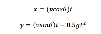
Here v is the initial velocity which we will keep constant, theta is the angle of launch which we will vary, and g is the gravitational constant which we will take as 9.81.

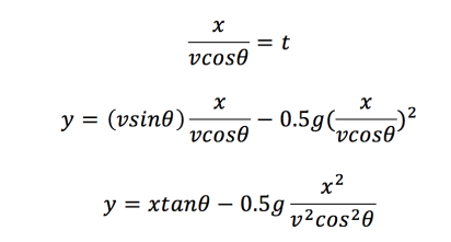
First let’s rearrange these equations to eliminate the parameter t.

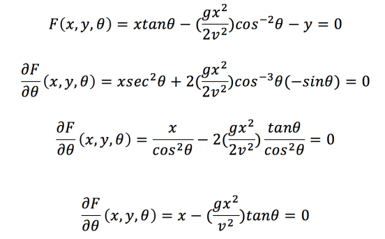
Next, we use the fact that the envelope of a curve is given by the points which satisfy the following 2 equations:

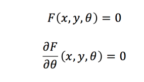
F(x,y,theta)=0 simply means we have rearranged an equation so that we have 3 variables on one side and have made this equal to 0.  The second of these equations means the partial derivative of F with respect to theta.  This means that we differentiate as usual with regards to theta, but treat x and y like constants.

Therefore we can rearrange our equation for y to give:

and in order to help find the partial differential of F we can write:

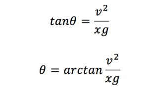
We can then rearrange this to get x in terms of theta:

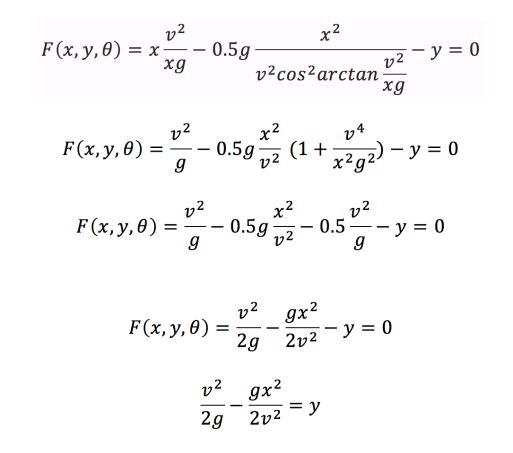
We can then substitute this into the equation for F(x,y,theta)=0 to eliminate theta:

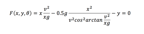
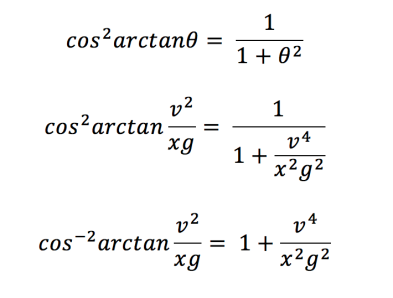
We then have the difficulty of simplifying the second denominator, but luckily we have a trig equation to help:

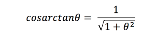
Therefore we can simplify as follows:

and so:

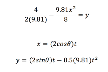
And we have our equation for the envelope of projectile motion!  As we can see it is itself a quadratic equation.  Let’s look at some of the envelopes it will create.  For example, if I launch a projectile with a velocity of 1, and taking g = 9.81, I get the following equation:

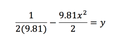
This is the envelope of projectile motion when I take the following projectiles in parametric form and vary theta from 0 to pi:

This gives the following graph:

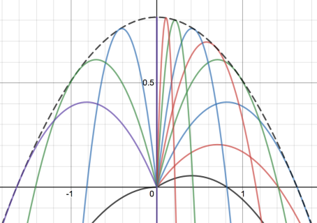
If I was to take an initial velocity of 2 then I would have the following:

And an initial velocity of 4 would generate the following graph:

So, there we have it, we can now create the equation of the envelope of curves created by projectile motion for any given initial velocity!

Other ideas for projectile motion

There are lots of other things we can investigate with projectile motion.  One example provided by fellow IB teacher Ferenc Beleznay is to fix the velocity and then vary the angle, then to plot the maximum points of the parabolas.  He has created a Geogebra app to show this:

You can then find that the maximum points of the parabolas lie on an ellipse (as shown below).

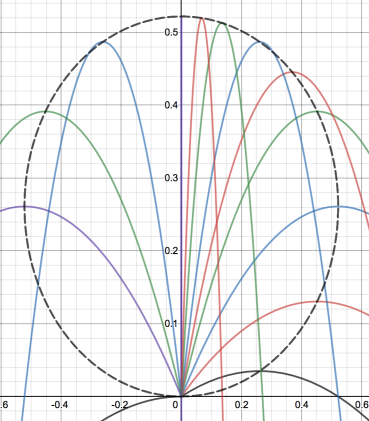
See if you can find the equation of this ellipse!