You are currently browsing the category archive for the ‘IB Maths’ category.

IB Maths Resources

On this site you will find IB Maths and IGCSE Maths Resources for IB Maths explorations and investigations. I’ve tried to build connections with real life maths, Theory of Knowledge (ToK) and ideas for maths careers. There are also maths videos, puzzles and lesson resources.  Scroll down to see more!

Intermathematics

Screen Shot 2023-04-07 at 11.09.42 AM

If you are a teacher then please also visit my new site.  This has been designed specifically for teachers of mathematics at international schools.  The content now includes over 3000 pages of pdf content for the entire SL/HL Analysis and SL/HL Applications syllabus Some of the content includes:

  1. Original pdf worksheets (with full worked solutions) designed to cover all the syllabus topics.  These make great homework sheets or in class worksheets – and are each designed to last between 40 minutes and 1 hour.
  2. Original Paper 3 investigations (with full worked solutions) to develop investigative techniques and support both the exploration and the Paper 3 examination.
  3. Over 150 pages of Coursework Guides to introduce students to the essentials behind getting an excellent mark on their exploration coursework.
  4. A large number of enrichment activities such as treasure hunts, quizzes, investigations, Desmos explorations, Python coding and more – to engage IB learners in the course.

There is also a lot more.  I think this could save teachers 200+ hours of preparation time in delivering an IB maths course – so it should be well worth exploring!

You can see some of examples of the content in the Teacher resources section of this site – which has a lot of worksheets and ideas for IB maths teachers.

Many thanks!
Andrew

One of the main benefits of flipping the classroom is allowing IB maths students to self-teach IB content. There are currently a good number of videos on youtube which allow students to self teach syllabus content, but no real opportunity to watch videos going through IB Higher Level past paper questions. So, I’ve started to put some of these together:

Playlist, Worked Exam Solutions:

The videos above are all around 10 minutes long and consist of talking through the solutions to 2-3 IB HL maths questions. The best way to use these videos is to pause the video at the start of the question, attempt it, then watch the video to check the answer and make notes on the method. Click on the top left hand corner to change the video being shown in the playlist.

The playlists below combine these worked solutions with the syllabus content videos, all grouped into the relevant syllabus strands:

Playlist 1, Algebra 1:

Sequences, Binomial, Logs, Induction, Permutations, Gaussian elimination:

Playlist 2, Complex numbers:

Converting from Cartesian to Polar, De Moivre’s Theorem, Roots of Unity:

Playlist 3: Functions:

Sketching graphs, Finding Inverses, Factor and Remainder Theorem, Sketching 1/f(x), sketching absolute f(x), translating f(x):

telephone2

The Telephone Numbers – Graph Theory

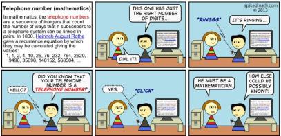
The telephone numbers are the following sequence:

1, 1, 2, 4, 10, 26, 76, 232, 764, 2620, 9496…

(where we start from n=0).

This pattern describes the total number of ways which a telephone exchange with n telephones can place a connection between pairs of people.

To illustrate this idea, the graph below is for n=4.  This is when we have 10 telephones:

telephone

Each red line represents a connection.  So the first diagram is for when we have no connections (this is counted in our sequence).  The next five diagrams all show a single connection between a pair of phones.  The last three diagrams show how we could have 2 pairs of telephones connected at the same time.  Therefore the 4th telephone number is 10.   These numbers get very large, very quickly.

Finding a recursive formula

The formula is given by the recursive relationship:

T(n) = T(n-1) + (n-1)T(n-2)

This means that to find (say) the 5th telephone number we do the following:

T(5) = T(5-1) + (5-1)T(5-2)

T(5) = T(4) + (4)T(3)

T(5) = 10 + (4)4

T(5) = 26

This is a quick way to work out the next term, as long as we have already calculated the previous terms.

Finding an nth term formula

The telephone numbers can be calculated using the nth term formula:


telephone7

 This is going to be pretty hard to derive!  I suppose the first step would start by working out the total number of connections possible between n phones – and this will be the the same as the graphs below:

telephone3

These clearly follow the same pattern as the triangular numbers which is 0.5(n² +n) when we start with n = 1.  We can also think of this as n choose 2 – because this gives us all the ways of linking 2 telephones from n possibilities.  Therefore n choose 2 also generates the triangular numbers.

But then you would have to work out all the permutations which were allowed – not easy!

Anyway, as an example of how to use the formula to calculate the telephone numbers, say we wanted to find the 5th number:

We have n = 5.  The summation will be from k = 0 and k = 2 (as 5/2 is not an integer).

Therefore T(5) = 5!/(20(5-0)!0!) + 5!/(21(5-2)!1!) + 5!/(22(5-4)!2!)

T(5) = 1 + 10 + 15 = 26.

Finding telephone numbers through calculus

Interestingly we can also find the telephone numbers by using the function:

y = e0.5x2+x

 and the nth telephone number (starting from n = 1)  is given by the nth derivative when x = 0.

For example,

telephone5

So when x = 0, the third derivative is 4.  Therefore the 3rd telephone number is 4.

The fifth derivative of the function is:

telephone6

So, when x =0 the fifth derivative is 26.  Therefore the 5th telephone number is 26.

If you liked this post you might also like:

Fermat’s Theorem on the Sum of two Squares – A lesser known theorem from Fermat – but an excellent introduction to the idea of proof.

Unbelievable: 1+2+3+4…. = -1/12 ? A result that at first glance looks ridiculous – and yet can be shown to be correct.  How?

circular inversion2

Circular inversions II

There are some other interesting properties of circular inversions.  One of which is that they preserve the “angle” between intersecting circles.  Firstly, how can circles have an angle between them?  Well, we draw 2 tangents to both the circles at the point of intersection, and then measure the angle between the 2 tangents:

circular inversion17

Therefore we can see that the “angle” between these 2 circles is 59.85 degrees.  If we then carry out a circular inversion we see the following:

circular inversion16

The inversion has been done with regards to the black circle centred around the origin.  The red and blue circles are mapped from outside the the black circle onto circles inside the black circle.  Now if we do the same as before – by finding the 2 tangents at the point of intersection, we find that the angle has remained the same – it is still 59.85 degrees.

It is also possible to find circles which remain unchanged under the inversion.  This happens when a circle is orthogonal (at a 90 degree angle) to the circle with which the inversion is being carried out.

circular inversion 18

The small circle has an angle of 90 degrees with the large circle, and therefore when we invert with respect to the large circle, we map the small circle onto itself.

The question is, why is all this useful?  Well, an entire branch of mathematics (non-Euclidean geometry) is concerned with being able to map points in our traditional Euclidean worldview (the geometry of high school triangles, parallel lines and circle theorems) to different geometrical systems entirely.  Circular inversion is a good introduction to this concept.

Also, circular inversion can sometimes make studying mathematical shapes easier to understand and explain.  For example, (from Wolfram):

circular inversion21

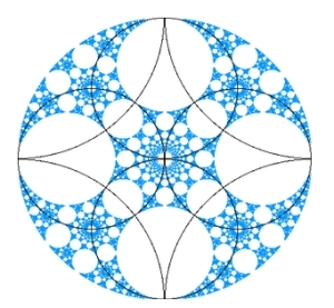
It would be very difficult to explain mathematically how the shape above is generated – whilst there are patterns, it is not obvious how to explain them. However, if we invert this shape through a circular inversion (with the circle at centre of the image) then we get the following:

circular inversion20

This is the image inside the circle – and now we can clearly see the pattern behind the generated image.  So, inversion has a lot of potential for simplifying geometrical problems.


SIR MODEL

If you are a teacher then please also visit my new site: intermathematics.com for over 2000+ pdf pages of resources for teaching IB maths!

Modelling Infectious Diseases

Using mathematics to model the spread of diseases is an incredibly important part of preparing for potential new outbreaks.  As well as providing information to health workers about the levels of vaccination needed to protect a population, it also helps govern first response actions when new diseases potentially emerge on a large scale (for example, Bird flu, SARS and Ebola have all merited much study over the past few years).

The basic model is based on the SIR model – this is represented by the picture above (from Plus Maths which has an excellent and more detailed introduction to this topic).  The SIR model looks at how much of the population is susceptible to infection, how many of these go on to become infectious, and how many of these go on to recover (and in what timeframe).

SIR MODEL2

Another important parameter is R0, this is defined as how many people an infectious person will pass on their infection to in a totally susceptible population.  Some of the R0values for different diseases are shown above.  This shows how an airbourne infection like measles is very infectious – and how malaria is exceptionally hard to eradicate because infected people act almost like a viral storage bank for mosquitoes.

One simple bit of maths can predict what proportion of the population needs to be vaccinated to prevent the spread of viruses.  The formula is:

VT = 1 – 1/R0

Where VT is the proportion of the population who require vaccinations. In the case of something like the HIV virus (with an R0 value of between 2 and 5), you would only need to vaccinate a maximum of 80% of the population.  Measles however requires around 95% vaccinations.  This method of protecting the population is called herd immunity

SIR MODEL 3
This graphic above shows how herd immunity works.  In the first scenario no members of the population are immunised, and that leads to nearly all the population becoming ill – but in the third scenario, enough members of the population are immunised to act as buffers against the spread of the infection to non-immunised people.

 \frac{dS}{dt} = - \beta I S
 \frac{dI}{dt} = \beta I S - \nu I
 \frac{dR}{dt} = \nu I

The equations above represent the simplest SIR (susceptible, infectious, recovered) model – though it is still somewhat complicated!

dS/dt represents the rate of change of those who are susceptible to the illness with respect to time.  dI/dt represents the rate of change of those who are infected with respect to time.  dR/dt represents the rate of change of those who have recovered with respect to time.

For example, if dI/dt is high then the number of people becoming infected is rapidly increasing.  When dI/dt is zero then there is no change in the numbers of people becoming infected (number of infections remain steady).  When dI/dt is negative then the numbers of people becoming infected is decreasing.

The constants β and ν are chosen depending on the type of disease being modelled.  β represents the contact rate – which is how likely someone will get the disease when in contact with someone who is ill.  ν is the recovery rate which is how quickly people recover (and become immune.

ν can be calculated by the formula:

D = 1/ν

where D is the duration of infection.

β can then be calculated if we know R0 by the formula:

R0 = β/ν

Modelling measles

So, for example, with measles we have an average infection of about a week, (so if we want to work in days, 7 = 1/ν and so ν = 1/7).   If we then take R0 = 15 then:

R0 = β/ν
15 = β/0.14
β = 2.14

Therefore our 3 equations for rates of change become:

dS/dt = -2.14 I S

dI/dt = 2.14 I S – 0.14 I

dR/dt = 0.14 I

Unfortunately these equations are very difficult to solve – but luckily we can use a computer program to plot what happens.   We need to assign starting values for S, I and R – the numbers of people susceptible, infectious, recovered (immune) from measles.  Let’s say we have a total population of 11 people – 10 who are susceptible, 1 who is infected and 0 who are immune.  This gives the following outcome:

SIR model 5

This shows that the infection spreads incredibly rapidly – by day 2, 8 people are infected.  By day 10 most people are immune but the illness is still in the population, and by day 30 the entire population is immune and the infection has died out.

SIR model 6

An illustration of just how rapidly measles can spread is provided by the graphic above.  This time we start with a population of 1000 people and only 1 infected individual – but even now, within 5 days over 75% of the population are infected.

SIR model 7

This last graph shows the power of herd immunity.  This time there are 100 susceptible people, but 900 people are recovered (immune), and there is again one infectious person.  This time the infection never takes off in the community – those who are already immune act as a buffer against infection.

If you enjoyed this post you might also like:

Differential Equations in Real Life – some other uses of differential equations in modelling predator-prey relationships between animal populations.

Essential Resources for IB Teachers

1) Intermathematics.com

Screen Shot 2021-08-21 at 1.07.49 PM

If you are a teacher then please also visit my new site.  This has been designed specifically for teachers of mathematics at international schools.  The content now includes over 2000 pages of pdf content for the entire SL and HL Analysis syllabus and also the SL Applications syllabus.  Some of the content includes:

  1. Original pdf worksheets (with full worked solutions) designed to cover all the syllabus topics.  These make great homework sheets or in class worksheets – and are each designed to last between 40 minutes and 1 hour.
  2. Original Paper 3 investigations (with full worked solutions) to develop investigative techniques and support both the exploration and the Paper 3 examination.
  3. Over 150 pages of Coursework Guides to introduce students to the essentials behind getting an excellent mark on their exploration coursework.
  4. A large number of enrichment activities such as treasure hunts, quizzes, investigations, Desmos explorations, Python coding and more – to engage IB learners in the course.

There is also a lot more.  I think this could save teachers 200+ hours of preparation time in delivering an IB maths course – so it should be well worth exploring!

Essential Resources for both IB teachers and IB students

1) Exploration Guides and Paper 3 Resources

Screen Shot 2021-12-01 at 1.19.14 PM

I’ve put together a 168 page Super Exploration Guide to talk students and teachers through all aspects of producing an excellent coursework submission.  Students always make the same mistakes when doing their coursework – get the inside track from an IB moderator!  I have also made Paper 3 packs for HL Analysis and also Applications students to help prepare for their Paper 3 exams.  The Exploration Guides can be downloaded here and the Paper 3 Questions can be downloaded here.

circular inversion2

Circular Inversion – Reflecting in a Circle

This topic is a great introduction to the idea of mapping – where one point is mapped to another.  This is a really useful geometrical tool as it allows complex shapes to be transformed into isomorphic (equivalent) shapes which can sometimes be easier to understand and work with mathematically.

One example of a mapping is a circular inversion.  The inversion rule maps a point P onto a point P’ according to the rule:

OP x OP’ = r2

To understand this, we start with a circle radius r centred on O.  The inversion therefore means that the distance from O to P multiplied by the distance from O to P’ will always give the constant value r2

circular inversion 3

This is an example of the circular inversion of the point A to the point A’.

We have the distance of OA as √2 and the radius of the circle as 2.  Therefore using the formula we can find OA’ by:

OA’ = r2 / OA = 4/√2

OA’ = 21.5. This means that the point A’ is a distance of 21.5 away from O on the same line as OA.

We can check that the Geogebra plot is correct – because this point A’ is plotted at (2,2) – which is indeed (using Pythagoras) a distance of 21.5 from O.

circular inversion 4

A point near to the edge of the circle will have an inversion also close to the circle

circular inversion 5

A point near to the centre will have an inversion a long way from the circle. The point (0,0) will be undefined as no point outside the circle will satisfy the inversion equation.

So, that is the basic idea behind circular inversion – though it gets a lot more interesting when we start inverting shapes rather than just points.

circular inversion 6

Circles through the origin map onto straight lines to infinity (see above).

circular inversion 7

Circles centred on the origin map to other circles centred on the origin (above).

circular inversion 10

Ellipses create these shapes (above).

circular inversion 11

The straight line through A B maps to a circle through the origin (above).

circular inversion 12

The solid triangle ABC maps to the pink region (above).

circular inversion 13

The solid square ABCD maps to the pink region (above).

These shapes can all be explored using the reflect object in circle button on Geogebra.

It is possible to extend the formula to 3 dimensions to give spherical inversion:

circular inversion 14

The above image is a 3D human head inverted in a sphere (from the Space Symmetry Structures website.  There’s lots to explore on this topic – it’s a good example of how art can be mathematically generated, as well as introducing isomorphic structures.

If you enjoyed this post you might also like:

The Riemann Sphere : Another form of mapping using spheres is the Riemann Sphere  – which is a way of mapping the entire complex plane to the surface of a sphere.

Fractals, Mandelbrot and the Koch Snowflake. Using maths to model infinite patterns.

Essential resources for IB students:

1) Exploration Guides and Paper 3 Resources

Screen Shot 2021-05-19 at 6.32.13 PM

I’ve put together four comprehensive pdf guides to help students prepare for their exploration coursework and Paper 3 investigations. The exploration guides talk through the marking criteria, common student mistakes, excellent ideas for explorations, technology advice, modeling methods and a variety of statistical techniques with detailed explanations. I’ve also made 17 full investigation questions which are also excellent starting points for explorations.  The Exploration Guides can be downloaded here and the Paper 3 Questions can be downloaded here.

polynomial roots

Graphically Understanding Complex Roots

If you have studied complex numbers then you’ll be familiar with the idea that many polynomials have complex roots. For example x2 + 1 = 0 has the solution x = i and -i.  We know that the solution to x2 – 1 = 0 ( x = 1 and -1) gives the two x values at which the graph crosses the x axis, but what does a solution of x = i or -i represent graphically?

There’s a great post on Maths Fun Facts which looks at basic idea behind this and I’ll expand on this in a little more detail.  This particular graphical method only works with quadratics:

Step 1

quadratic1

You have a quadratic graph with complex roots, say y = (x – 1)2 + 4. Written in this form we can see the minimum point of the graph is at (1,4) so it doesn’t cross the x axis.

Step 2

quadratic2

Reflect this graph downwards at the point of its vertex. We do this by transforming y = (x – 1)2 + 4 into y =  -(x – 1)2 + 4

Step 3

quadratic3

We find the roots of this new equation using the quadratic formula or by rearranging – leaving the plus or minus sign in.
-(x – 1)2 + 4 = 0
(x-1) = ± 2
x = 1 ± 2

Plot a circle with centre (1,0) and radius of 2.  This will touch both roots.

Step 4

Graphically Understanding complex roots

We can now represent the complex roots of the initial equation by rotating the 2 real roots we’ve just found 90 degrees anti-clockwise, with the centre of rotation the centre of the circle.

The points B and C on the diagram are a representation of the complex roots (if we view the graph as representing the complex plane).  The complex roots of the initial equation are therefore given by x = 1 ± 2i.

General case

It’s relatively straightforward to show algebraically what is happening:

If we take the 2 general equations:

1) y = (x-a)2 + b
2) y = -(x-a)2 + b  (this is the reflection at the vertex of equation 1 )

(b > 0 ).  Then the first equation will always have complex roots.  The roots of both equations will be given by:

1) a ±i√b

2) a ±√b

So we can think of (2) as representing a circle of radius √b, centred at (a,0).  Therefore multiplying √b by i has the effect of rotating the point (√b, 0 ) 90 degrees anti-clockwise around the point (a,0).  Therefore the complex roots will be graphically represented by those points at the top and bottom of this circle.  (a, √b) and (a, -√b)

Graphically finding complex roots of a cubic

There is also a way of graphically calculating the complex roots of a cubic with 1 real and 2 complex roots.  This method is outlined with an algebraic explanation here

Step 1

cubic1

We plot a cubic with 1 real and 2 complex roots, in this case y = x3 – 9x2 + 25x – 17.

Step 2

Graphically Understanding complex roots

We find the line which goes through the real root (1,0) and which is also a tangent to the function.

Step 3

Graphically Understanding complex roots

If the x co-ordinate of the tangent intersection with the cubic is a and the gradient of the tangent is m, then the complex roots are a ± (√m)i.  In this case the tangent x intersection is at 4 and the gradient of the tangent is 1, therefore the complex roots are 4 ± 1i.

[2nd last sentence edited – thanks for the comments below!]

Essential resources for IB students:

1) Exploration Guides and Paper 3 Resources

Screen Shot 2021-05-19 at 6.32.13 PM

I’ve put together four comprehensive pdf guides to help students prepare for their exploration coursework and Paper 3 investigations. The exploration guides talk through the marking criteria, common student mistakes, excellent ideas for explorations, technology advice, modeling methods and a variety of statistical techniques with detailed explanations. I’ve also made 17 full investigation questions which are also excellent starting points for explorations.  The Exploration Guides can be downloaded here and the Paper 3 Questions can be downloaded here.

This is the British International School Phuket’s IB maths exploration page. This list is primarily for IB Maths Applications SL students (exam in 2021 onwards).  If you are doing IB Maths Analysis (exam in 2021 onwards) then go to this page instead.  Scroll down for the full list of possible topics and ideas!

Essential resources for IB students:

1) Revision Village

Screen Shot 2021-05-19 at 9.55.51 AM

Revision Village has been put together to help IB students with topic revision both for during the course and for the end of Year 12 school exams and Year 13 final exams.  I would strongly recommend students use this as a resource during the course (not just for final revision in Y13!) There are specific resources for HL and SL students for both Analysis and Applications.

Screen Shot 2018-03-19 at 4.42.05 PM.png

There is a comprehensive Questionbank takes you to a breakdown of each main subject area (e.g. Algebra, Calculus etc) and then provides a large bank of graded questions.  What I like about this is that you are given a difficulty rating, as well as a mark scheme and also a worked video tutorial.  Really useful!

Screen Shot 2021-05-19 at 10.05.18 AM

The Practice Exams section takes you to a large number of ready made quizzes, exams and predicted papers.   These all have worked solutions and allow you to focus on specific topics or start general revision.  This also has some excellent challenging questions for those students aiming for 6s and 7s.

Each course also has a dedicated video tutorial section which provides 5-15 minute tutorial videos on every single syllabus part – handily sorted into topic categories.

2) Exploration Guides and Paper 3 Resources

Screen Shot 2021-05-19 at 6.32.13 PM

I’ve put together four comprehensive pdf guides to help students prepare for their exploration coursework and Paper 3 investigations. The exploration guides talk through the marking criteria, common student mistakes, excellent ideas for explorations, technology advice, modeling methods and a variety of statistical techniques with detailed explanations. I’ve also made 17 full investigation questions which are also excellent starting points for explorations.  The Exploration Guides can be downloaded here and the Paper 3 Questions can be downloaded here.

Maths Studies and Applications IA Exploration Topics

Make sure you read the Maths Studies guidance from the IB prior to starting your IA maths exploration – this linked site gives the full list of assessment criteria you will be judged against and also gives 9 full examples of investigations students have done.

Given the assessment criteria it’s probably easiest to conduct a data analysis investigation, though you can choose to explore other parts of the syllabus instead.  To get good marks make sure you carefully follow the marking criteria points given by the IB and try and personalise your investigation as much as possible.  Be innovative, choose something you are interested in and enjoy it!

Primary or Secondary data? 

The main benefit of primary data is that you can really personalise your investigation.  It allows you scope to investigate something that perhaps no-one else has ever done.  It also allows you the ability to generate data that you might not be able to find online.  The main drawback is that collecting good quality data in sufficient quantity to analyze can be time consuming.    You should aim for an absolute minimum of 50 pieces of data – and ideally 60-100 to give yourself a good amount of data to look at.

The benefits of secondary data are that you can gain access to good quality raw data on topics that you wouldn’t be able to collect data on personally – and it’s also much quicker to get the data.  Potential drawbacks are not being able to find the raw data that fits what you  want to investigate – or sometimes having too much data to wade through.

Secondary data sources:

1) The Census at School website is a fantastic source of secondary data to use.  If you go to the random data generator you can download up to 200 questionnaire results from school children around the world on a number of topics (each year’s questionnaire has up to 20 different questions).

2) If you’re interested in sports statistics then the Olympic Database is a great resource.  It contains an enormous amount of data on winning times and distances in all events in all Olympics.  Follow links at the top of the page to similar databases on basketball, golf, baseball and American football.

3) If you prefer football you can also find a lot of football stats on the Who Scored website.  This gives you data on things like individual players’ shots per game, pass completion rate etc.

4) The World Bank has a huge data bank – which you can search by country or by specific topic.  You can compare life-expectancy rates, GDP, access to secondary education, spending on military, social inequality, how many cars per 1000 people and much much more.

5) Gapminder is another great resource for comparing development indicators – you can plot 2 variables on a graph (for example urbanisation against unemployment, or murder rates against urbanisation) and then run them over a number of years. You can also download Excel speadsheets of the associated data.

6) Wolfram Alpha is one of the most powerful maths and statistics tools available – it has a staggering amount of information that you can use.  If you go to the examples link above, then you can choose from data on everything from astronomy, the human body, geography, food nutrition, sports, socioeconomics, education and shopping.

7) Plotly is a great visual graphic site – you can create visually interesting infographics and analyse data from hundreds of other sources.

8) TSM – the Technology for Secondary  Mathematics is something of an internet dinosaur – but has a great deal of downloadable data files on everything from belly-button ratios to lottery number analysis and baby weights.

9) Google Public Data – an enormous source for public data, which is displayed graphically and can be searched.

10) Nationmaster – another huge site with pretty much any statistic and data comparing countries.  Currently they have 19 million data points – so you’re likely to find something useful!

11) Google word usage analysis – a great tool which allows you to track the usage of words over the centuries.

Example Maths Studies IA Investigations:

Some of these ideas taken from the excellent Oxford IB Maths Studies textbook.

Correlations:

1) Is there a correlation between hours of sleep and exam grades?

Studies have shown that a good night’s sleep raises academic attainment.
2) Is there a correlation between height and weight?
The NHS use a chart to decide what someone should weigh depending on their height. Does this mean that height is a good indicator of weight?

3) Is there a correlation between arm span and foot height?
This is also a potential opportunity to discuss the Golden Ratio in nature.

4) Is there a correlation between the digit ratio and maths ability?
Studies show there is a correlation between digit ratio and everything from academic ability, aggression and even sexuality.

5) Is there a correlation between smoking and lung capacity?

6) Is there a correlation between GDP and life expectancy?
Run the Gapminder graph to show the changing relationship between GDP and life expectancy over the past few decades.

7) Is there a correlation between numbers of yellow cards a game and league position?
Use the Guardian Stats data to find out if teams which commit the most fouls also do the best in the league.

8) Is there a correlation between Olympic 100m sprint times and Olympic 15000m times?
Use the Olympic database to find out if the 1500m times have go faster in the same way the 100m times have got quicker over the past few decades.

9) Is there a correlation between sacking a football manager and improved results?
A recent study suggests that sacking a manager has no benefit and the perceived improvement in results is just regression to the mean.

10) Is there a correlation between time taken getting to school and the distance a student lives from school?

11) Does eating breakfast affect your grades?

12) Is there a correlation between stock prices of different companies?
Use Google Finance to collect data on company share prices.

13) Does teenage drinking affect grades?
A recent study suggests that higher alcohol consumption amongst teenagers leads to greater social stress and poorer grades.

14) Is there a correlation between unemployment rates and crime?
If there are less work opportunities, do more people turn to crime?

15) Is there a correlation between female participation in politics and wider access to further education?

16) Is there a correlation between blood alcohol laws and traffic accidents?

17) Is there a correlation between height and basketball ability?

18) Is there a correlation between stress and blood pressure?

19) Is there a correlation between Premier League wages and league positions?

Normal distributions:

1) Are a sample of student heights normally distributed?
We know that adult population heights are normally distributed – what about student heights?

2) Are a sample of flower heights normally distributed?

3) Are a sample of student weights normally distributed?

4) Are a sample of student reaction times normally distributed?
Conduct this BBC reaction time test to find out.

5) Are a sample of student digit ratios normally distributed?

6) Are the IB maths test scores normally distributed?
IB test scores are designed to fit a bell curve. Investigate how the scores from different IB subjects compare.

7) Are the weights of “1kg” bags of sugar normally distributed?

Other statistical investigations

1) Does gender affect hours playing sport?
A UK study showed that primary school girls play much less sport than boys.

2) Investigation into the distribution of word lengths in different languages.
The English language has an average word length of 5.1 words.  How does that compare with other languages?

3) Do bilingual students have a greater memory recall than non-bilingual students?
Studies have shown that bilingual students have better “working memory” – does this include memory recall?

4) Investigation about the distribution of sweets in packets of Smarties.  A chance to buy lots of sweets!  Also you could link this with some optimisation investigation.

5) 22) Using Chi Squared to crack codes – Chi squared can be used to crack Vigenere codes which for hundreds of years were thought to be unbreakable. Unleash your inner spy!

6) Which times tables do students find most difficult to learn? – Are some calculations like 7×8 harder than others?  Why?

Modelling using calculus

1) How can you optimise the area of a farmer’s field for a given length of fence?
A chance to use some real life maths to find out the fence sides that maximise area.

2) Optimisation in product packaging.  
Product design needs optimisation techniques to find out the best packaging dimensions.

Probability and statistics

1) The probability behind poker games

2) Finding expected values for games of chance in a casino.

3) Birthday paradox:
The birthday paradox shows how intuitive ideas on probability can often be wrong.  How many people need to be in a room for it to be at least 50% likely that two people will share the same birthday? Find out!

4)  Which times tables do students find most difficult?
A good example of how to conduct a statistical investigation in mathematics.

5) Handshake problem
With n people in a room, how many handshakes are required so that everyone shakes hands with everyone else?

Other ideas

If you want to do an investigation with a bit more mathematical content then have a look at this page for over 300 ideas for Maths SL and HL students.

poker

This post is based on the fantastic PlusMaths article on bluffing– which is a great introduction to this topic.  If you’re interested then it’s well worth a read.  This topic shows the power of mathematics in solving real world problems – and combines a wide variety of ideas and methods – probability, Game Theory, calculus, psychology and graphical analysis.

You would probably expect that there is no underlying mathematical strategy for good bluffing in poker – indeed that a good bluffing strategy would be completely random so that other players are unable to spot when a bluff occurs.  However it turns out that this is not the case.

As explained by John Billingham in the PlusMaths article, when considering this topic it helps to really simplify things first.  So rather than a full poker game we instead consider a game with only 2 players and only 3 cards in the deck (1 Ace, 1 King, 1 Queen).

The game then plays as follows:
1) Both players pay an initial £1 into the pot.
2) The cards are dealt – with each player receiving 1 card.
3) Player 1 looks at his card and can:
(a) check
(b) bet an additional £1
4) Player 2 then can respond:
a) If Player 1 has checked, Player 2 must also check.  This means both cards are turned over and the highest card wins.
b) If Player 1 has bet £1 then Player 2 can either match (call) that £1 bet or fold.  If the bets are matched then the cards are turned over and the highest card wins.

So, given this game what should the optimal strategy be for Player 1? An Ace will always win a showdown, and a Queen always lose – but if you have a Queen and bet, then your opponent who may only have a King might decide to fold thinking you actually have an Ace.

In fact the optimal strategy makes use of Game Theory – which can mathematically work out exactly how often you should bluff:

poker2

This tree diagram represents all the possible outcomes of the game.  The first branch at the top represents the 3 possible cards that Player 2 can be dealt (A,K,Q) each of which have a probability of 1/3.  The second branch represents the remaining 2 possible cards that Player 1 has – each with probability 1/2.  The numbers at the bottom of the branches represent the potential gain or loss from betting strategies for Player 2 – this is calculated by comparing the profit/loss relative to if both players had simply shown their cards at the beginning of the game.

For example, Player 2 has no way of winning any money with a Queen – and this is represented by the left branch £0, £0.  Player 2 will always win with an Ace.  If Player 1 has a Queen and bluffs then Player 2 will call the bet and so will have gained an additional £1 of his opponents money relative to a an initial game showdown (represented by the red branch).  Player 1 will always check with a King (as were he to bet then Player 2 would always call with an Ace and fold with a Queen) and so the AK branch also has a £0 outcome relative to an initial showdown.

So, the only decisions the game boils down to are:

1) Should Player 1 bluff with a Queen? (Represented with a probability of b on the tree diagram )
2) Should Player 2 call with a King?  (Represented with a probability of c on the tree diagram ).

Now it’s simply a case of adding the separate branches of the tree diagram to find the expected value for Player 2.

The right hand branch (for AQ and AK) for example gives:

1/3 . 1/2 . b . 1
1/3 . 1/2 . (1-b) . 0
1/3 . 1/2 . 0

So, working out all branches gives:

Expected Value for Player 2 = 0.5b(c-1/3) – c/6
Expected Value for Player 1 = -0.5b(c-1/3) + c/6

(Player 1’s Expected Value is simply the negative of Player 2’s. This is because if Player 2 wins £1 then Player 1 must have lost £1). The question is what value of b (Player 1 bluff) should be chosen by Player 1 to maximise his earnings?  Equally, what is the value of c (Player 2 call) that maximises Player 2’s earnings?

It is possible to analyse these equations numerically to find the optimal values (this method is explained in the article), but it’s more mathematically interesting to investigate both the graphical and calculus methods.

Graphically we can solve this problem by creating 2 equations in 3D:

z = 0.5xy-x/6 – y/6

poker7

z = -0.5xy+x/6 + y/6

poker8

In both graphs we have a “saddle” shape – with the saddle point at x = 1/3 and y = 1/3.  This can be calculated using Wolfram Alpha. At the saddle point we have what is known in Game Theory as a Nash equilibrium – it represents the best possible strategy for both players.   Deviation away from this stationary point by one player allows the other player to increase their Expected Value.

Therefore the optimal strategy for Player 2 is calling with precisely c = 1/3 as this minimises his loses to -c/6 = -£1/18 per hand.  The same logic looking at the Expected Value for Player 1 also gives b = 1/3 as an optimal strategy.  Player 1 therefore has an expected value of +£1/18 per hand.

We can arrive at the same conclusion using calculus – and partial derivatives.

z = 0.5xy-x/6 – y/6

For this equation we find the partial derivative with respect to x (which simply means differentiating with respect to x and treating y as a constant):

zx = 0.5x – 1/6

and also the partial derivative with respect to y (differentiate with respect to y and treat x as a constant):

zy = 0.5y -1/6

We then set both of these equations to 0 and solve to find any stationary points.

0 = 0.5x – 1/6
0 = = 0.5y -1/6
x = 1/3 y = 1/3

We can then see that this is a saddle point by using the formula:

D = zxx . zyy – (zxy)2

(where zxx means the partial 2nd derivative with respect to x and zxy means the partial derivative with respect to x followed by the partial derivative with respect to y. When D < 0 then we have a saddle point).

This gives us:

D = 0.0 – (0.5)2 = -0.25

As D < 0 then we have a saddle point – and the optimal strategy for both players is c= 1/3 and b = 1/3.

We can change the rules of the game to see how this affects the strategy.  For example, if the rules remain the same except that players now must place a £1.50 bet (with the initial £1 entry still intact) then we get the following equation:

Player 2 Expected Value = b/12(-1+7c) – 3c/12

This has a saddle point at b = 3/7, c = 1/7.  So the optimal strategy is 3/7 bluffing and 1/7 calling.  If Player 2 calls more than 3/7 then Player 1 can never bluff (b = 0), leaving Player 2 with a negative Expected Value.  If Player 2 calls less than 3/7 then Player 1 can always bluff (b = 1).

If you enjoyed this you might also like:

The Gambler’s Fallacy and Casino Maths – using maths to better understand casino games

Game Theory and Tic Tac Toe – using game theory to understand games such as noughts and crosses

Essential resources for IB students:

1) Exploration Guides and Paper 3 Resources

Screen Shot 2021-05-19 at 6.32.13 PM

I’ve put together four comprehensive pdf guides to help students prepare for their exploration coursework and Paper 3 investigations. The exploration guides talk through the marking criteria, common student mistakes, excellent ideas for explorations, technology advice, modeling methods and a variety of statistical techniques with detailed explanations. I’ve also made 17 full investigation questions which are also excellent starting points for explorations.  The Exploration Guides can be downloaded here and the Paper 3 Questions can be downloaded here.

Joh-RiemannSphere01

The Riemann Sphere

The Riemann Sphere is a fantastic glimpse of where geometry can take you when you escape from the constraints of Euclidean Geometry – the geometry of circles and lines taught at school.  Riemann, the German 19th Century mathematician, devised a way of representing every point on a plane as a point on a sphere.  He did this by first centering a sphere on the origin – as shown in the diagram above.  Next he took a point on the complex plane (z = x + iy ) and joined up this point to the North pole of the sphere (marked W).  This created a straight line which intersected the sphere at a single point at the surface of the sphere (say at z’).  Therefore every point on the complex plane (z) can be represented as a unique point on the sphere (z’) – in mathematical language, there is a one-to-one mapping between the two.  The only point on the sphere which does not equate to a point on the complex plane is that of the North pole itself (W).  This is because no line touching W and another point on the sphere surface can ever reach the complex plane.  Therefore Riemann assigned the value of infinity to the North pole, and therefore the the sphere is a 1-1 mapping of all the points in the complex plane (and infinity).

Riemann 2

So what does this new way of representing the two dimensional (complex) plane actually allow us to see?  Well, it turns on its head our conventional notions about “straight” lines.  A straight line on the complex plane is projected to a circle going through North on the Riemann sphere (as illustrated above).  Because North itself represents the point at infinity, this allows a line of infinite length to be represented on the sphere.

riemann sphere

Equally, a circle drawn on the Riemann sphere not passing through North will project to a circle in the complex plane (as shown in the diagram above).  So, on the Riemann sphere – which remember is isomorphic (mathematically identical) to the extended complex plane, straight lines and circles differ only in their position on the sphere surface.  And this is where it starts to get really interesting – when we have two isometric spaces there is no way an inhabitant could actually know which one is his own reality.  For a two dimensional being living on a Riemann sphere,  travel in what he regarded as straight lines would in fact be geodesic (a curved line joining up A and B on the sphere with minimum distance).

By the same logic, our own 3 dimensional reality is isomorphic to the projection onto a 4 dimensional sphere (hypersphere) – and so our 3 dimensional universe is indistinguishable from a a curved 3D space which is the surface of a hypersphere.  This is not just science fiction – indeed Albert Einstein was one to suggest this as a possible explanation for the structure of the universe.  Indeed, such a scenario would allow there to be an infinite number of 3D universes floating in the 4th dimension – each bounded by the surface of their own personal hypersphere.  Now that’s a bit more interesting than the Euclidean world of straight lines and circle theorems.

If you liked this you might also like:

Imagining the 4th Dimension. How mathematics can help us explore the notion that there may be more than 3 spatial dimensions.

The Riemann Hypothesis Explained. What is the Riemann Hypothesis – and how solving it can win you $1 million

Are You Living in a Computer Simulation? Nick Bostrom uses logic and probability to make a case about our experience of reality.

Essential resources for IB students:

1) Exploration Guides and Paper 3 Resources

Screen Shot 2021-05-19 at 6.32.13 PM

I’ve put together four comprehensive pdf guides to help students prepare for their exploration coursework and Paper 3 investigations. The exploration guides talk through the marking criteria, common student mistakes, excellent ideas for explorations, technology advice, modeling methods and a variety of statistical techniques with detailed explanations. I’ve also made 17 full investigation questions which are also excellent starting points for explorations.  The Exploration Guides can be downloaded here and the Paper 3 Questions can be downloaded here.

Website Stats

  • 9,480,431 views

About

All content on this site has been written by Andrew Chambers (MSc. Mathematics, IB Mathematics Examiner).

New website for International teachers

I’ve just launched a brand new maths site for international schools – over 2000 pdf pages of resources to support IB teachers.  If you are an IB teacher this could save you 200+ hours of preparation time.

Explore here!

Free HL Paper 3 Questions

P3 investigation questions and fully typed mark scheme.  Packs for both Applications students and Analysis students.

Available to download here

IB Maths Super Exploration Guide

A Super Exploration Guide with 168 pages of essential advice from a current IB examiner to ensure you get great marks on your coursework.

Available to download here.

Recent Posts

Follow IB Maths Resources from Intermathematics on WordPress.com