Sierpinski Triangle: A picture of infinity

Sierpinski Triangle: A picture of infinity

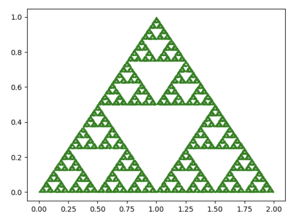
This pattern of a Sierpinski triangle pictured above was generated by a simple iterative program.  I made it by modifying the code previously used to plot the Barnsley Fern. You can run the code I used on repl.it.  What we are seeing is the result of 30,000 iterations of a simple algorithm.  The algorithm is as follows:

Transformation 1:

x_i+1 = 0.5x_i

y_i+1= 0.5y_i

Transformation 2:

x_i+1 = 0.5x_i + 0.5

y_i+1= 0.5y_i+0.5

Transformation 3:

x_i+1 = 0.5x_i +1

y_i+1= 0.5y_i

So, I start with (0,0) and then use a random number generator to decide which transformation to use.  I can run a generator from 1-3 and assign 1 for transformation 1, 2 for transformation 2, and 3 for transformation 3.   Say I generate the number 2 – therefore I will apply transformation 2.

x_i+1 = 0.5(0) + 0.5

y_i+1= 0.5(0)+0.5

and my new coordinate is (0.5,0.5).  I mark this on my graph.

I then repeat this process – say this time I generate the number 3.  This tells me to do transformation 3.  So:

x_i+1 = 0.5(0.5) +1

y_i+1= 0.5(0.5)

and my new coordinate is (1.25, 0.25).  I mark this on my graph and carry on again.  The graph above was generated with 30,000 iterations.

Altering the algorithm

We can alter the algorithm so that we replace all the 0.5 coefficients of x and y with another number, a.

a = 0.3 has disconnected triangles:

When a = 0.7 we still have a triangle:

By a = 0.9 the triangle is starting to degenerate

By a = 0.99 we start to see the emergence of a line “tail”

By a = 0.999 we see the line dominate.

And when a = 1 we then get a straight line:

When a is greater than 1 the coordinates quickly become extremely large and so the scale required to plot points means the disconnected points are not visible.

If I alternatively alter transformations 2 and 3 so that I add b for transformation 2 and 2b for transformation 3 (rather than 0.5 and 1 respectively) then we can see we simply change the scale of the triangle.

When b = 10 we can see the triangle width is now 40 (we changed b from 0.5 to 10 and so made the triangle 20 times bigger in length):

Fractal mathematics

This triangle is an example of a self-similar pattern – i.e one which will look the same at different scales.  You could zoom into a detailed picture and see the same patterns repeating.  Amazingly fractal patterns don’t fit into our usual understanding of 1 dimensional, 2 dimensional, 3 dimensional space.  Fractals can instead be thought of as having fractional dimensions.

The Hausdorff dimension is a measure of the “roughness” or “crinkley-ness” of a fractal.  It’s given by the formula:

D = log(N)/log(S)

For the Sierpinski triangle, doubling the size (i.e S = 2), creates 3 copies of itself (i.e N =3)

This gives:

D = log(3)/log(2)

Which gives a fractal dimension of about 1.59.  This means it has a higher dimension than a line, but a lower dimension than a 2 dimensional shape.